Why Subsea Annotation Is Different
Most people working in computer vision have been trained, formally or informally, on datasets drawn from well-lit, high-contrast scenes: object detection on COCO or ImageNet, lane segmentation on road footage, defect detection in factory inspection images. These datasets share a characteristic that subsea footage does not: consistent, controlled illumination.
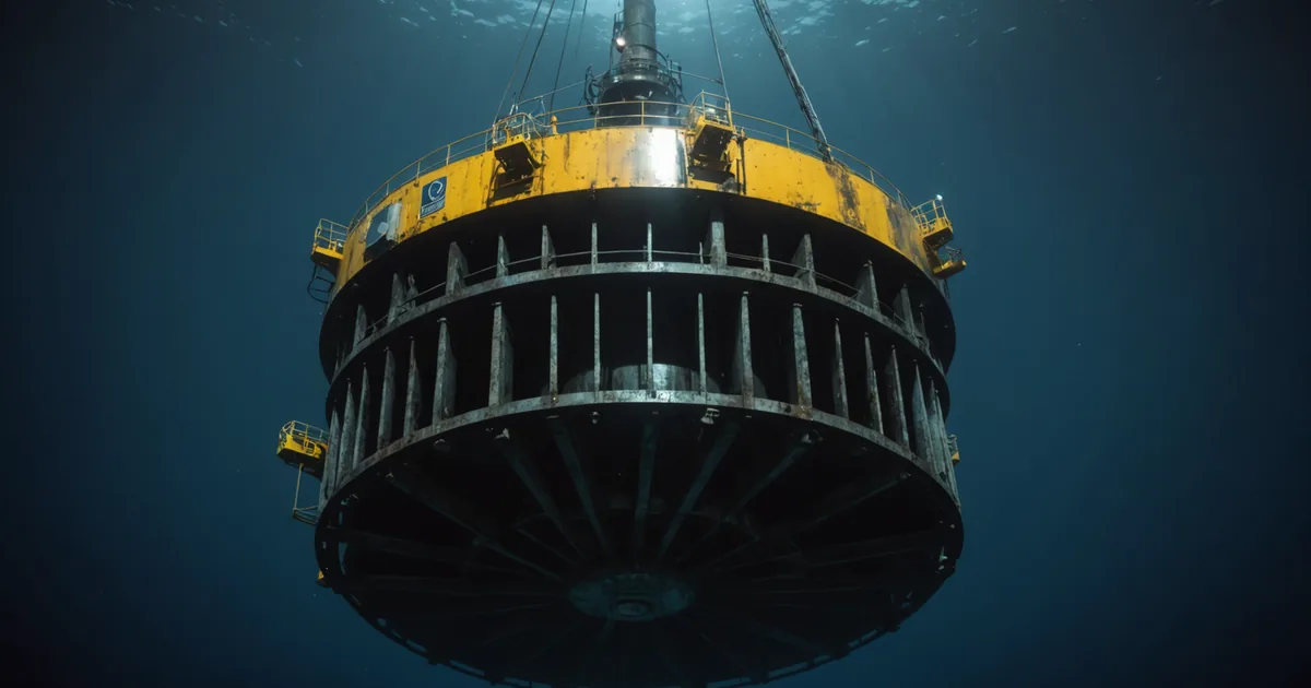
ROV inspection footage is captured by a camera mounted on a vehicle moving through water at typical depths of 15 to 60 metres. The illumination is provided by LED floodlights mounted on the ROV, positioned close to the camera. This creates strong specular reflections on wet steel surfaces, deep shadows in structural recesses, and a rolling lighting angle as the ROV traverses the structure. The same corroded surface zone can look orange-brown and clearly degraded when the ROV approaches directly, and appear flat grey with no obvious texture anomaly when the ROV passes at a shallower angle with the light washing across rather than illuminating the surface face-on.
Turbidity adds another layer of variability. Particle loading in the water column scatters the ROV floodlights and reduces contrast. In North Sea summer conditions, biofouling season creates dense marine growth on structure surfaces that partially or wholly obscures the underlying steel. In winter, turbidity from storm resuspension can reduce effective visibility to less than a metre. The same structure surveyed in August and January may produce footage with dramatically different visual characteristics, and both need to return useful detection output.
The Annotation Problem
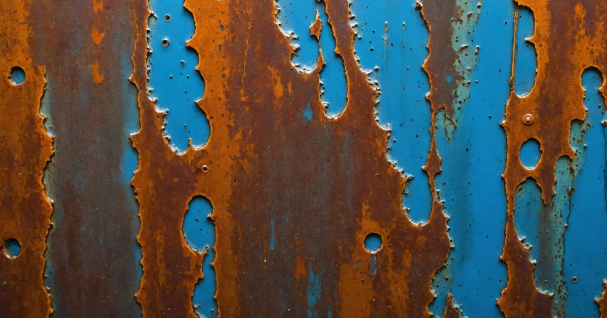
Building a training dataset requires expert annotators who can look at a video frame and correctly label what they see. For standard object detection datasets, annotators can be trained reasonably quickly on clear categorical definitions. Corrosion on subsea steel is not a clear categorical definition. It is a spectrum from surface oxidation (intact coating with slight discolouration) through active pitting (visible corrosion product, local steel loss) to advanced surface attack (substantial wall loss, structural concern). Where on that spectrum a given frame sits requires judgment that takes years to develop in the offshore inspection context.
We are not saying it requires a chartered engineer to annotate every frame. What it requires is an annotator who has enough inspection experience to distinguish: active corrosion product from iron staining left by previous corrosion that is now inhibited; marine growth from surface coating degradation (both can appear as irregular patches at distance); and mechanical damage from corrosion-driven surface loss (both appear as material absence but have different maintenance implications).
Our early annotation approach used qualified inspection engineers to label the initial dataset. This produced high-quality ground truth but was expensive and slow. We then moved to a tiered system: a trained annotation team handles first-pass labelling using a detailed visual reference guide we developed from the initial engineer-annotated set, and a subset of each annotation batch goes to an inspection engineer for quality review and correction. The corrections feed back into the reference guide and are used to recalibrate the annotation team's thresholds over time.
Handling Lighting Variance in the Dataset
Lighting variance is the single largest source of annotation inconsistency in our dataset. An annotator looking at a strongly lit face-on frame of a corroded zone will correctly label it. The same annotator looking at an oblique-lit frame of the same zone a few seconds later in the footage may not recognise it as the same defect type, because the visual cues are different. This creates class label noise that, if uncorrected, teaches the model the wrong thing: it learns to associate certain lighting artifacts with corrosion rather than learning the underlying surface characteristics that indicate corrosion.
We addressed this partly through dataset curation and partly through augmentation. Curation involved reviewing frame sequences for the same structure zone across different lighting conditions and ensuring consistent labelling within those sequences. Where a zone was clearly labelled correctly in a good-lighting frame, we confirmed or corrected its label in the adjacent degraded-lighting frames rather than treating each frame in isolation.
Augmentation involved systematically varying the brightness, contrast, colour temperature, and scattering characteristics of training images to force the model to learn features that are stable across lighting conditions rather than features that vary with lighting. Underwater scattering augmentation specifically, simulating the fog effect of high-turbidity water, proved important for generalisation to winter survey conditions where our initial model had degraded performance.
Class Imbalance Across Defect Types
Clean structure with no anomalies is the most common condition in offshore wind inspection footage. Most foundations, most of the time, are in good condition. This creates a class imbalance in naturally collected footage: examples of acceptable surface condition vastly outnumber examples of each defect type. A model trained naively on this distribution will learn to predict "no defect" because that is almost always correct, and will perform poorly on the defect classes that actually matter.
Handling this requires intentional dataset construction. We oversample from footage where defects are present, we collect specifically from older assets and from sections of foundations known to have higher degradation rates, and we supplement with expert-annotated still images from industry reference materials. The goal is not to match real-world prevalence in the training set, but to give the model sufficient examples of each defect type to learn reliable discriminative features.
The rarest classes in our dataset are structural cracks and cathodic protection wear indicators. Genuine structural cracks in modern offshore wind monopiles are uncommon in the asset age range we are working with: most North Sea wind installations are less than 15 years old and well within expected structural design life. But the detection of cracks is the highest-consequence finding type, and under-representation in training data is a serious limitation. We flag this explicitly in our confidence scoring: crack detections carry a higher false positive rate than corrosion detections, and we communicate that to engineers reviewing the outputs.
Annotator Calibration Over Time
One thing that surprised us about building inspection annotation teams is how much annotator calibration drifts over time without active intervention. An annotation team that is well-calibrated at the start of a project will gradually develop shared interpretations that diverge from the original reference definitions, particularly for borderline cases. This is a natural outcome of people working together and converging on pragmatic shared judgments. The problem is that the convergent pragmatic judgment may not match what an independent inspection engineer would call the correct label.
We now run monthly calibration sessions where a random sample of previously annotated frames is reviewed by the annotation team and an inspection engineer together. Disagreements are resolved and the resolution rationale is documented. Over six months of doing this, we have seen annotation consistency measured by inter-annotator agreement on borderline cases improve substantially, and the distance between annotation team judgment and inspection engineer judgment on the same frames decrease. This is ongoing work, not a problem that gets solved once.
The output quality of detection models in this domain is fundamentally constrained by the quality of the annotation process. It is not enough to collect footage and run it through a labelling tool. The annotation has to be grounded in real inspection expertise, systematically maintained, and honest about where uncertainty exists. In our dataset, every annotation carries a confidence level set by the annotator. Frames with low-confidence annotations are tracked separately and used carefully in training, with higher weight given to high-confidence examples.